Quantize, Don't Truncate
Liquid AI shipped LFM2.5-Embedding-350M — a 350-million-parameter embedding model small enough to run on a laptop CPU. It looks like a good fit for on-device search. But the model card is silent on the thing you need to know before you build an index with it: how small can the vectors get before search quality falls apart?
Worse, it advertises no Matryoshka support — the training trick that lets you chop a vector in half and have it still work. Models built for compression usually publish a table showing what you keep at each size. This one publishes nothing. Neither does anyone else: I went looking, and there are zero published vector-quantization numbers for any LFM2.5 model. Everything circulating under names like "LFM2.5 INT8" or "Q4" is weight quantization — shrinking the model, not the vectors it produces. Different axis, different question.
So I measured it. It compresses unusually well, and the missing Matryoshka support turns out not to matter — because quantizing all 1024 dimensions beats truncating to fewer, at a fraction of the bytes.
The thing being compressed
A quick level-set, because two different things get called "quantization" and conflating them will cost you a week.
An embedding model turns a chunk of text into a list of numbers — a vector. This model emits 1024 numbers per chunk, each a 32-bit float. That's 4,096 bytes per chunk. Search works by storing a vector for every chunk in your corpus and, at query time, comparing the query's vector against all of them.
The storage adds up faster than people expect. A million chunks at 4KB each is 4GB, and you generally want that in RAM, because the whole point is scanning it fast. Ten million chunks is 40GB, and now you're renting a much larger machine.
Vector quantization is storing those 1024 numbers in fewer bits each. Instead of a 32-bit float per dimension, use 8 bits, or 4, or 1. At 1 bit per dimension you're keeping only the sign of each number — positive or negative — and 1024 bits is 128 bytes. That's 32× smaller than where you started.
Weight quantization — shrinking the model file itself, which is what a GGUF "Q4_K_M" download is — is a separate lever. It changes how much RAM the encoder needs and how fast it runs. It does not change the size of your index. Both are worth doing; this post is entirely about the first one.
How to read the chart
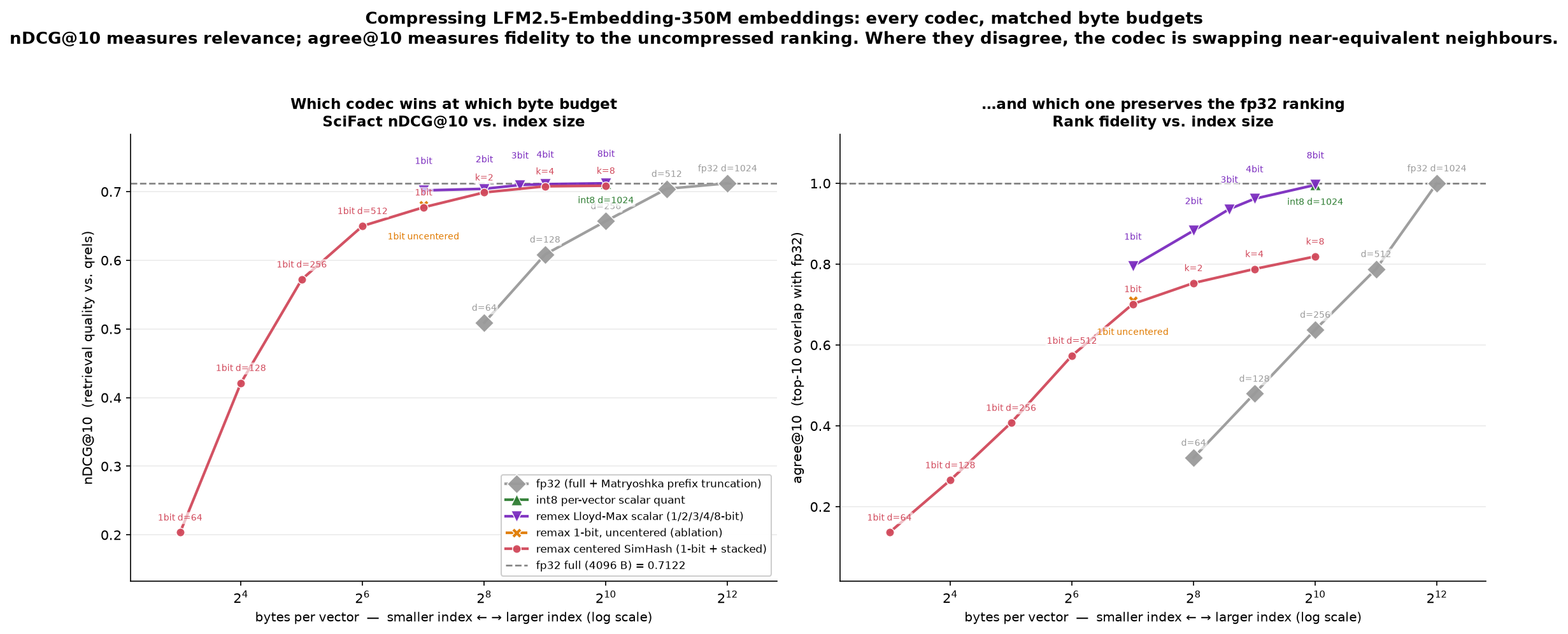
This is the whole result in one picture.
The x-axis is bytes per vector — your storage bill. It runs from 4,096 bytes on the right (uncompressed) down to 8 bytes on the left. It's a log scale, so each step left is a halving. Left is cheaper.
The y-axis on the left panel is nDCG@10 — search quality. If that acronym is unfamiliar: it's a score from 0 to 1 for "how good are the top 10 results," where getting the right answer at position 1 counts for more than getting it at position 10. It's the standard retrieval metric. Higher is better. You do not need to know how it's computed to read this chart; you need to know that 0.71 is a good score on this dataset and 0.50 is a bad one.
The dashed horizontal line is uncompressed quality. That's the target. A point sitting on the dashed line is losing nothing.
So: you want points in the upper left. High quality, low storage. And the curve runs flat along the dashed line from 4,096 bytes all the way down to 128 bytes, then falls off a cliff. Everything between those two points is nearly free compression. You are paying almost nothing in quality for a 32× reduction in storage.
The right-hand panel plots something subtler, and it's there because it's the honest counterweight to the left panel. It measures agreement: of the 10 results uncompressed search would have returned, how many does the compressed index return? That number declines steadily as you compress — it does not stay flat. At 128 bytes the compressed index agrees with only about 80% of the uncompressed top 10.
Both panels are true at once. Compression is reshuffling your results — it just reshuffles among documents that were about equally good, so the quality score doesn't notice. That's fine if you're feeding a RAG pipeline. It's not fine if you promised someone deterministic, reproducible result ordering. Know which one you're building.
The numbers
Test corpus is BEIR SciFact: 5,183 scientific abstracts, 300 real queries, 339 human relevance judgments. Uncompressed baseline scores 0.7122, which is where a competent small retriever should land — for reference, e5-base-v2 gets 0.7194 and bge-base 0.7434 on the same task. That the number came out in the right range is the evidence the encoder was driven correctly.
| Storage | vs. uncompressed | Method | nDCG@10 | Quality kept |
|---|---|---|---|---|
| 4,096 B | 1× | float32 (baseline) | 0.7122 | 100% |
| 1,024 B | 4× | int8 | 0.7122 | 100.0% |
| 512 B | 8× | 4-bit | 0.7110 | 99.8% |
| 384 B | 10.7× | 3-bit | 0.7097 | 99.6% |
| 256 B | 16× | 2-bit | 0.7042 | 98.9% |
| 128 B | 32× | 1-bit | 0.7018 | 98.5% |
| 64 B | 64× | 1-bit, half the dims | 0.6501 | 91.3% |
| 32 B | 128× | 1-bit, quarter dims | 0.5722 | 80.3% |
int8 is free. Four times smaller, and the score is identical to four decimal places. If you are storing float32 embeddings from this model today and doing nothing else, this is a no-brainer.
1-bit costs 1.5%. 32× smaller for a rounding error. Your million-chunk index just went from 4GB to 128MB.
The part that surprised me
Here's why the missing Matryoshka support doesn't bite.
Matryoshka training (the nesting-doll trick) teaches a model to put its most important information in the first dimensions, so you can throw away the back half of every vector and still search well. It's the standard answer to "my index is too big." Models trained for it publish truncation tables. LFM2.5 doesn't do this, which is what made me expect trouble.
But truncation is not the only way to make vectors smaller. You can cut dimensions — or you can keep all the dimensions and store each one in fewer bits. Those are different axes, and on this model they are wildly unequal:
| Approach | Storage | nDCG@10 |
|---|---|---|
| float32, truncated to 256 dims | 1,024 B | 0.6572 |
| 1-bit, all 1024 dims | 128 B | 0.7018 |
Eight times less storage and 6.8% better quality. Cutting dimensions is the expensive way to save space here. Cutting precision is nearly free.
And the truncation numbers do confirm the missing Matryoshka is real — this model degrades three to seven times faster under truncation than jina-v3, which is trained for it, depending on how far you cut. At a quarter of its dimensions LFM2.5 loses 7.7% where jina-v3 loses 1.1%; at a sixteenth it's 28.5% against 10.2%. The caveat in the model card is accurate. It just doesn't bind, because truncation is the wrong lever to reach for.
Which generalizes to a rule of thumb: when an embedding model doesn't advertise Matryoshka support, that's an argument for quantizing harder, not for giving up on a small index.
Getting the last 1.5% back
Nobody deploys the compressed codes alone. The standard pattern is two-stage: scan the small index to get a shortlist, then re-rank just that shortlist using exact vectors fetched from disk. The index stays in RAM and stays tiny; you pay full precision on a handful of rows instead of the whole corpus.
How big does the shortlist need to be? On this model, startlingly small:
| Shortlist from the 128-byte index | nDCG@10 | vs. uncompressed |
|---|---|---|
| none — compressed only | 0.6772 | 95.1% |
| re-rank top 10 | 0.7044 | 98.9% |
| re-rank top 25 | 0.7131 | 100% |
| re-rank top 50 | 0.7137 | 100% |
Twenty-five rows out of 5,183 fully recovers uncompressed quality over a 32×-smaller index. The published conventions for this — Elasticsearch's BBQ, Qdrant's guidance — suggest fetching 3–4× your result count as a shortlist. Here 2.5× was enough.
(The 100% entries land a hair above baseline. That's noise on a 300-query test set, not a free lunch — re-ranking a shortlist can break ties favorably. Read it as "recovered," not "improved.")
Predicting it in advance
Which compression scheme wins is not a property of the scheme. It's a property of the model's output geometry, and it flips between models. On a previous corpus (SPECTER2, a specialized science-paper encoder) 1-bit beat 2-bit and 3-bit — an inversion that makes no sense until you look at how the vectors are shaped. On LFM2.5 the ordering is the textbook one. Same code, opposite curves.
So before running any search benchmark, I measured the geometry and wrote down a prediction. The useful statistic is how evenly the model spreads information across its dimensions after a random rotation. A model that spreads it evenly (a ratio near 1.0) suits multi-bit schemes; a lopsided one (SPECTER2 measured 0.39) does not. LFM2.5 measured 0.937 — nearly ideal — and the prediction that followed from it held at every single storage budget.
Worth recording: a different and more obvious geometry statistic would have gotten this wrong. Measuring how concentrated the model's output is in a few directions suggested 11.6% effective dimensionality — strongly lopsided, predict the opposite. It's the post-rotation number that's predictive, not the raw spread. The rotation fixes lopsidedness that the naive measurement is still counting.
Two things I predicted that didn't hold, recorded because negative results are the ones people quietly drop: centering the vectors before 1-bit encoding was supposed to help and didn't (0.6808 uncentered vs 0.6772 centered — marginally worse, within noise), and my own centering heuristic is therefore unvalidated and flagged as such in the code. And my first instinct, before measuring anything, was that 1024 dimensions was too thin for binary quantization to work well. It wasn't.
If you're deploying this model
- Use int8. 4× smaller, zero measured cost. There is no argument against it.
- Consider 1-bit with a top-25 rescore. 32× smaller with a shortlist pass that fully recovers quality. This is the configuration I'd ship.
- Don't truncate dimensions. On this model it's strictly worse than quantizing — more storage and lower quality.
- Pin
transformers < 5.12. A plainpip install transformersgets 5.14 today and dies on the first forward pass withTypeError: _noncausal_shortconv_forward() got an unexpected keyword argument 'seq_idx'. The model's custom code patches internals that moved. This cost me a run. - Don't skip the prompt prefixes. Queries need
"query: "and documents need"document: ". Liquid warns that omitting them silently degrades quality, and "silently" is the operative word — you get plausible-looking vectors and quietly worse search.
Follow-up: one explanation here was wrong
The table above has two codecs at 128 bytes scoring 0.7018 and 0.6772, and I explained the gap as one codec simply being better than the other. That was wrong, and I went and measured it properly: the difference was that the losing one binarized the search query as well as the documents. Keeping the query in full precision closes almost the entire gap, costs no storage, and turned out to be worth more than doubling the index.
The compression numbers in this post stand — what changed is the reason for them. Written up in Don't Binarize the Query.
Caveats
One dataset, one random seed, 300 queries. Differences smaller than about 0.005 nDCG aren't resolvable here — the ordering of the compression schemes is solid, the exact percentages are not. SciFact is English-only and scientific prose; LFM2.5 is a 15-language model and I tested none of the other fourteen. Documents were cut at the model's 512-token limit. The encoder ran at full precision, so weight quantization stacks on top of this independently and is untested here.
And the honest framing: this is one corpus. The whole point of the geometry section is that these curves are model-specific and don't transfer. Run the measurement on your own data before trusting a number from someone else's.
Everything is in the repo
The harness, the raw results, the figure, and the prediction-registered-in-advance are all in oaustegard/remax#53:
bench/geometry.py— the geometry diagnostic and its predictionbench/embed_lfm25.py— encoding (83 minutes for 5,183 abstracts on four CPU cores)bench/eval_lfm25.py— the compression comparisonbench/rerank_lfm25.py— the two-stage sweepbench/results/LFM25_SUMMARY.md— the write-up with every number
The model is also wired up as a packable embedder for remax_kb, so you can build a single-file portable index with it.